Statistical Theories to detect Sideways Markets

 

Introduction

When the financial securities go through the horizontal price movement for the notable period of time, change in volatility is noticeable by traders and the market is often described as Sideways Market. Sideways Market is one of the various facets of the Financial market. They appear as frequently as the trending market. Several interesting characteristics of the Sideways Market can be high value for both traders and academic communities in the related field. For the financial traders, Sideways Market can serve as the good entry timing in a view that the low volatility during Sideways Market should clear up in the near future and they should lead to the birth of new trending period. The trend direction can change from the previous trend but they might just continue the old one. Whichever direction the trend follows, new high volatility period can provide the good opportunities for traders.  For the academic community, the phenomenon of the Sideways Market further confirms the observations of clustering behaviour of volatility and they might be highly related to the causation of the clustering behaviours. On the other hand, many existing econometrics and time series forecasting tools do not address Sideways Market separately although the properties of Sideways Market is different from the trending market. Therefore this might provide new research opportunity for the interesting discoveries for the statistics or econometrics researchers. In spite of such high appearances in the historical data, the available studies on Sideways Market are very few. There are not many choices for the methodology in identifying Sideways Market. Previously many traders used the Average Directional Index (ADX) to detect Sideways Market. However, just like other technical indicators, ADX uses an averaging algorithm and they are lagging behind actual signal. Many false entry signals can confuse traders causing them financial losses. Besides the ADX indicators, other approaches to identify the Sideways Market are not well established. In this article, we introduce three statistical approaches to identify Sideways Market. The three approaches include the trinomial tree model approach, volatility approach and high low range approach. These three approaches are relatively simple to implement and so they can be easily included as the part of the systematic trading algorithm. In the next section, we will introduce the concept of these approaches. To provide better understanding, we also supply simple models for each approach created in MS-Excel Spreadsheet visualizing the calculation steps.

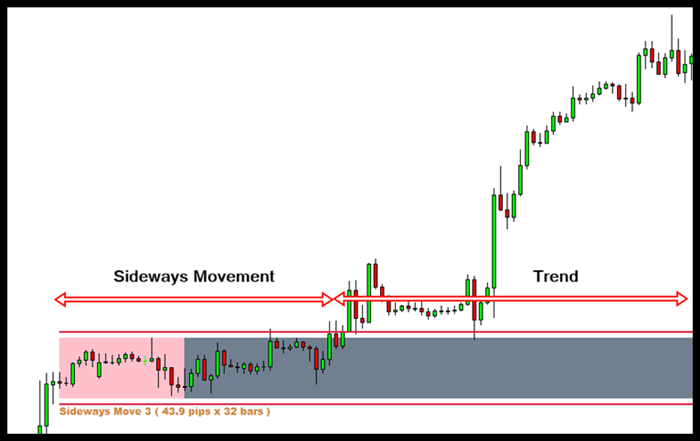
Figure 1  Sideways Market and Trend Market

Trinomial Tree Approach

Tree based methods is very popular tools to value many financial assets due to their easy implementation. Binomial trees and trinomial trees are the two popular variations of the tree based methods. With the simple binomial tree model, the price is assumed to either go up or go down. The assumptions of the simple binomial tree exclude the chance that the price might stay at the same price. For our purpose to study Sideways Market, the simple binomial tree model is rather limited as we can’t model the horizontal price movement. Alternatively, with the simple trinomial tree model, the price is assumed to either go up or go down or stay at the same price. As three movements are possible than two, the trinomial tree model can be more accurate in describing Sideways market than binomial tree model. In Figure 2, we show how the starting price at node S (1, 1) evolves through each time step. To further demonstrate the concept, we created the 5 step (5 candle bars) trinomial tree model in Figure 2 in our spreadsheet. In our simple 5 step trinomial model, we first assigned the equal probability 0.333 to going up, going down and lateral movement and we generated terminating probabilities at each node (Figure 3).  Then for the comparison purpose, we created another model with the assigned probabilities of 0.4, 0.4 and 0.2 respectively to going up, going down and lateral movement (Figure 4). Depending on the probability profile, the terminating probabilities for each price at the end of time period is different. Assigning smaller probability to the lateral movement, we get narrow terminating probability zone in the middle nodes of trinomial tree model. To detect sideways market, we need to decide the cut probability around the centre node of our trinomial tree model. This trinomial model approach can be easily extended towards many time steps. The advantage of this model is that the model does not require historical price data. Therefore, this is a useful approach when there is only limited data. The disadvantage of this approach is that it takes up quite large memory space when the time steps gets bigger. To create the n step trinomial model, we need a matrix with 2n+1 row and n+1 column. For example, for 100 steps trinomial model, we need two matrices of 201 rows and 101 columns to store the terminating prices and terminating probabilities respectfully.

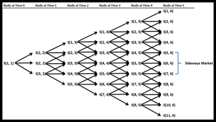
Figure 2  Trinomial Tree Model for 5 time step where S(i, j) = node of price i at time j

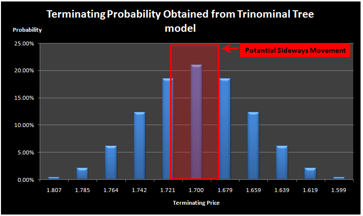
 Figure 3  Terminating probabilities at each price node for 5 step trinomial tree model when equal probabilities are assigned

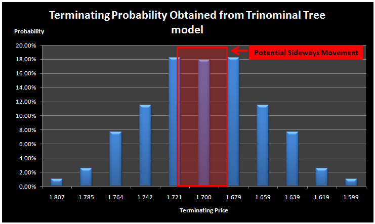
Figure 4  Terminating probabilities at each price node for 5 step trinomial tree model when non equal probabilities are assigned

 

Volatility Approach

As Sideways Market can be characterized by the horizontal price movements, such a price pattern can be described using low volatility during the period. To detect Sideways Market using volatility, we need to examine the volatility of current market and compare it to the historical volatilities. In another words, we need to construct distribution of price variance through historical data. It is well known fact that the sampling distribution of sample variance follow the chi squared distribution for the normally distributed samples. Two possible approaches to construct the distribution of sample variance include the simulation and historical construction approaches. For the simplicity, we constructed the distribution with historical construction approach for the 1000 EURUSD price observations. Also we directly calculate distribution of standard deviation instead of variance to save few steps. In the first step, we calculated the standard deviation for the first 20 candle bars and rolled the calculation forward the most recent observations. Then we constructed the frequency and probability tables. For the comparison purpose, we repeated the same steps for 30 candle bars and 40 candles bars. From Figure 5, 6 and 7, we can observe that the distribution of standard deviation is non normal and close to the chi squared distribution. Therefore, there is a tendency that sample standard deviation is more densely clustered around the lower quartile range of the standards deviation. Depending on what the cut probability is assigned, the emergent point of Sideways Market can differ. However, for demonstration purpose, we have marked first two lowest columns as the low volatility Sideways Movement in Figure 5, 6 and 7. For trading purpose, the sensible cut probability must be chosen. In comparison to the trinomial tree model, volatility approach has the advantage of having fewer parameters. In the trinomial tree model, users required to find out sensible probability for going up, going down and lateral movements as well as the cut probability. For volatility approach, users are only required to find out the cut probability and length of Sideways Market. Disadvantage of the volatility approach is that the model accuracy is dependent on the constructed frequency and probability distribution table. Therefore, user must construct the distribution of sample standards deviation on the sufficiently large historical data.

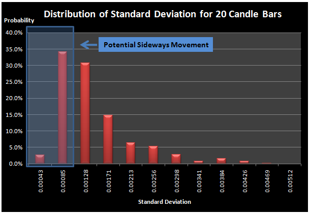
Figure 5  Distribution of Standard Deviation for 20 candle bars

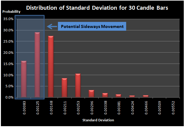
Figure 6  Distribution of Standard Deviation for 30 candle bars

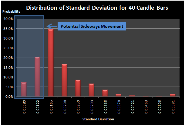
 Figure 7  Distribution of Standard Deviation for 40 candle bars

 

High Low Range Approach

We also introduce one more alternative approach using the high low range of the market.  This approach is similar to the volatility approach in a way that it needs to construct the frequency and probability distribution table. Instead of calculating standard deviation over historical price, we calculate the high low range of the historical prices. The high low range is calculated by subtracting the highest price among high price series from the lowest price among the low price series. For this article, we have constructed the frequency and probability distribution tables for 20, 30 and 40 candle bars for the 1000 EURUSD price observations. As shown in Figure 8, 9 and 10, the distribution of the high low range is quite similar to the distribution of the standard deviation in the volatility approach. Just like the volatility approach, the high low range approach requires only few inputs from users including the cut probability and length of Sideways Market. The main difference from the volatility approach is that the high low range approach does not concern other candle bars except the highest price and lowest price candle bars taken for the range calculation whereas the volatility approach concerns all the candle bars within the period of the Sideways Market and their deviation from the mean are contributed toward the value of the standard deviation.

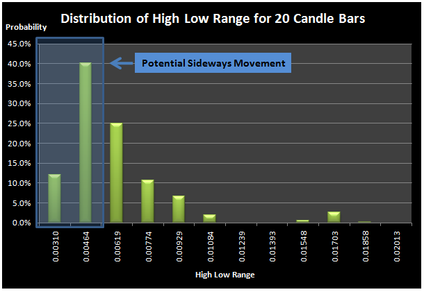
Figure 8  Distribution of High Low Range for 20 candle bars 

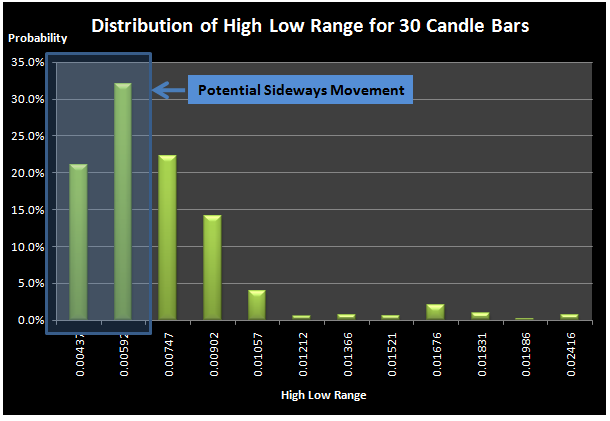
Figure 9  Distribution of High Low Range for 30 candle bars

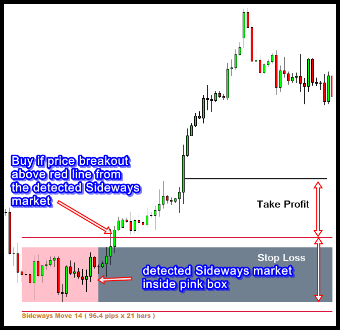
Figure 10  Distribution of High Low Range for 40 candle bars  

Trading Strategy with Sideways Market

The trading strategy with Sideways Market is relatively simple. The most important assumption for traders is that the market will have high volatility trending period in the near future as we had the low volatility market for the sufficiently long period of time in the past. Therefore, the most frequently used trading strategy involves the market entry based on the price breakout. Once the Sideways Market is detected, traders can place their buy order above the top of the Sideways Market.  Likewise, traders can place their sell order below the bottom of the Sideways Market.  When the order is placed, it is important to place orders with some distance from the boxes to prevent that order is executed over false breakout. To demonstrate this concept, we show the detected Sideways Market from the historical data and the future price movements after the appearance of the Sideways Market. The Sideways Market is marked by the pink box in Figure 11 and 12. In the classic setup, for the buy entry (Figure 11), traders can place their take profit at the box height from the top of the box and the bottom of the box can be the stop loss level for the buy entry. Likewise, for the sell entry, traders can place their take profit below at the box height from the bottom of the box and the top of the box can be the stop loss level for the sell entry (Figure 12). Of course, with modern backtesting technology, the take profit and stop loss level can be finely tuned for different financial securities.

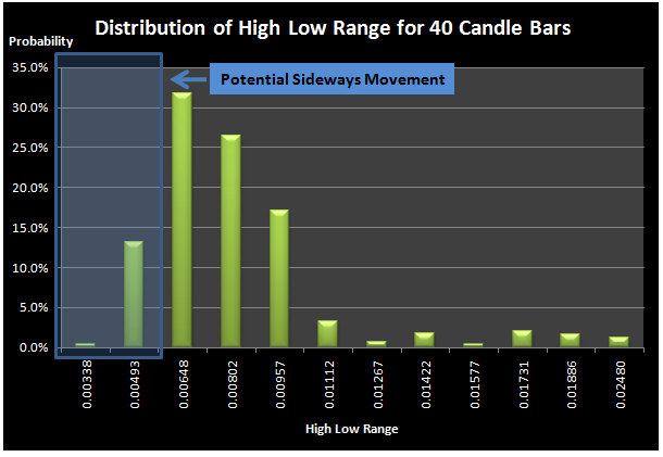
Figure 11  Classic buy entry set up for the detected Sideways Market

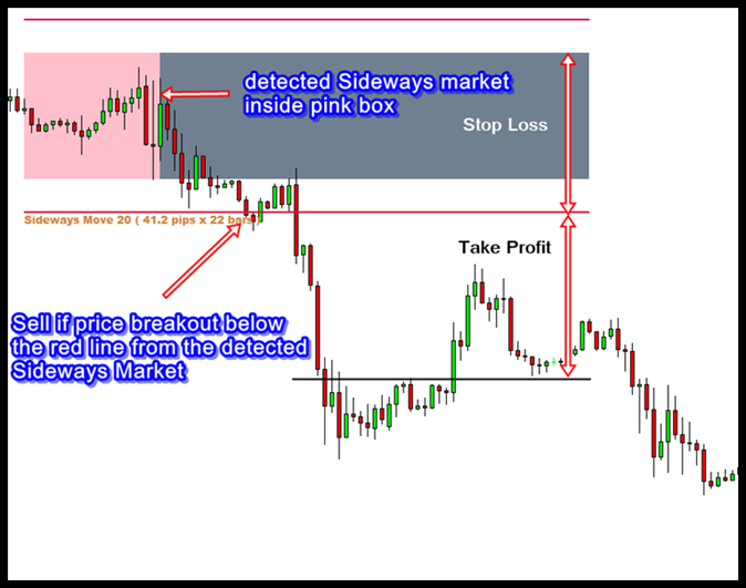
 Figure 12  Classic sell entry set up for the detected Sideways Market

 

Conclusion

The long low volatility period during Sideways Market can serve as the good entry timing for traders. Therefore, traders can develop a good trading strategy based on Sideways Market identification. The average Directional Index (ADX) indicator is often used among traders to detect Sideways Market. However, the ADX indicator’s lagging property is well known due to its averaging algorithm.  At the moment, there are no other well established approaches to detect Sideways Market. In this article, we have introduced three alternative approaches based on the statistical characteristics of Sideways Market. The three alternative approaches include the trinomial tree approach, volatility approach and high low range approach. Throughout this article, we have demonstrated the concept of each approach and we also provided the simple model created on the MS Excel Spreadsheet.  Finally we have provided a demonstration of a simple trading strategy based on the detection of Sideways Market for traders.

 

References

Boyle, P. P., 1986. ‘‘Option Valuation Using a Three-Jump Process.’’International Options Journal, Vol. 3, pp. 7–12.

Derman, E., I. Kani, and N. Chriss., 1996. ‘‘Implied Trinomial Trees of the Volatility Smile.’’ Journal of Derivatives, Vol. 4, No. 3, pp. 7–22.

Lee, C. F., Lee J. C. and Lee, A.C., 2013. “Statistics for Business and Financial Economics”. New York: Springer.

Pesavento, L. and Jouflas, L., 2007. “Trade what you see: How to profit from pattern recognition”. New Jersey: John Wiley & Sons, Inc.

Rouah, F. D. and Vainberg, G., 2007. “Option Pricing Models &Volatility Using Excel-VBA”. New York: John Wiley & Sons, Inc.